Day: April 4, 2018

Suppose a star emits a photon. Its wave function spreads over space, perhaps over light years.

On a far planet, a poet is looking at the night sky: if they  see that photon they will be inspired to write a great poem. Meanwhile at the other edge of the galaxy there is a pig, also, for its own porcine reasons, gazing skywards, and the photon wave function also passes through its retina. The pig may see the photon or the poet may see the photon. (Or, of course, it may be seen by neither.)  But it absolutely cannot be seen by both of them. If the photon materialises in an eyeball of one, it cannot do so in an eyeball of the other.  The wave function collapses, instantaneously and simultaneously across all space.

This rings alarm bells. The Theory of Relativity tells us loud and clear that ‘simultaneity’ is a dirty word, but it really does apply here. The arrival of the photon wave function at the pig and the poet may be simultaneous in the picture above, but there will be reference frames in which it arrives at the pig before the poet, and frames where the poet comes before the pig. Whatever frame you’re working in, the wave function collapse is simultaneous everywhere in that frame.

It’s the truly spooky bit of quantum mechanics that really nobody understands. An object – be it a photon, an electron, an atom, or a cat – has a wave function, and we can study the behaviour of that wave function by solving complicated differential equations. Then a measurement is made of some property, and the wave function changes randomly but instantly into a state where that property is defined. If the wave function is ‘real’ it defies relativity. If it is not ‘real’ then what is?

Most physicists solve this puzzle by ignoring it – the so-called ‘shut up and calculate’ school. I’m not going to explain the puzzle here – nobody can. What I do want to do is show that it is not really new, but linked to an older one.

Let’s introduce a logical formalism for discussing the collapse of the wave function in an ordered and well-defined way.  This was done by John von Neumann in his “Mathematical Foundations of Quantum Mechanics”, (Springer 1932, English translation by R T Beyer, Princeton, 1955) and what follows is his development, with modernised notation.

We need to introduce a neat concept called the density matrix.  This combines the two sorts of uncertainty that we have to deal with: quantum uncertainty and the established uncertainty of statistics and thermodynamics.

First, from quantum mechanics we take the idea of a basis set of states |i>, which are eigenstates of some measurement operator  (so Â |i> = a_i|i>). In what follows I’ll use as an example the simple case where there are just two states describing the spin of an electron as up |↑> or down |↓>;  they could also be the states |x> of delta functions at particular positions, or the pure sine wave states |p> that have definite wavelength and thus definite momentum.

Secondly, from Statistical Mechanics we take the idea of a large ensemble of N states |ν>, which are the actual states of many systems in equilibrium with one another.  The  |ν> states are (in general) not the same as the |i> states but they can be written in terms of them: |ν> = Σ_i <i|ν>  |i>, because the |i> states are a basis set. <i|ν>  is a number, the i-component of the ν state in the ensemble.

Right, that’s the apparatus in place. The density matrix is just the average over the ensemble of the Cartesian product of the components

ρ_ij=(¹/_N) Σ_ν <i|ν> <ν|j>

What can you do with it? Well the diagonal elements ρ_ii correspond to the average over the ensemble of | <ν|i> |², which, according to the Born interpretation, is the probability of finding state |ν> in state |i> if you measure it with  . It tells us the probability of getting the result a_i where the probability includes both the quantum uncertainty and the statistical uncertainty from the ensemble.

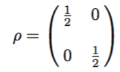
Let’s take an example.  If we take an ensemble of many electrons of which half are spin up and half are spin down then the matrix has ¹/₂  on each diagonal element and the off-diagonals are zero, because each    |ν> is either up or down, so the product of  <ν|↑> and <ν|↓> is always zero.  The diagonal tells us that if you pick an electron at random from the ensemble, there’s a 50% chance each for it being spin up or spin down.

Now let’s get a bit less trivial. We’ll take a sample of spin-down electrons, all the same this time,  and then rotate them 90 degrees about the y axis, so they point in the +x direction.

These states give the density matrix which has the same diagonal elements as the last one, but non-zero off-diagonal elements. The diagonal elements tell us that there is, again, a 50:50 chance of detecting the electron in an up or down state, though this time it’s because of quantum uncertainty.

If the diagonal elements give the probabilities, you might wonder whether there’s any point to the off-diagonal elements. But they do play a part. Suppose that, for both examples, we rotate the spins buy another 90 degrees before we measure them.  Under a rotation R the density matrix becomes  ρ’=RρR^†. A bit of  matrix arithmetic shows the matrix for the first example is unchanged, on the second example, the sideways states, is

which is obvious, with hindsight. The second rotation converts the spin direction from the x to the z axis,  so they will always be in the spin up state if you measure them, whereas for the first example the result is still 50:50 unpredictable.

So the density matrix encompasses quantum uncertainties, which may become certain if you ask a different question, and statistical uncertainties which cannot.  Diagonal elements give probabilities and off-diagonal elements contain information on the degree of quantum coherence. If you want to know more about it, try Feynman’s textbook  “Statistical Mechanics: a set of lectures” (CRC press, 1998).

As time goes by the states will evolve, and the evolution of the density matrix has the apparently simple form ρ’=e^-iHt/ℏ ρ e^iHt/ℏ. I say ‘apparently simple’ because H, which is being exponentiated, is a matrix. But this is standard quantum mechanics and the techniques exist to handle it. The |i> wave functions  oscillate at their characteristic frequencies.

But the matrix can also describe the effect of a measurement of the quantity corresponding to the operator Â. The measurement asks of each state |ν > which of the |i> basis states it belongs to: if it is in one of those states it stays in it, if it is in a superposition then it will drop into one of the|i>, the probability for each being   |<i|ν >|².  So the density matrix becomes ρ’_ij= δ_ij ρ_ij. The diagonal elements are preserved, and all the off-diagonal elements vanish, as each member of the ensemble is now in a definite basis state.

To say ‘a measurement zeroes all the off-diagonal terms of the density matrix’ expresses the ‘collapse of the wave function’ correctly and completely, but in a smooth and non-sensational way.

These two equations,  ρ’=e^-iHt/ℏ ρ e^iHt/ℏ and ρ’_ij= δ_ij ρ_ij, both describe how a system changes with time. They are different because the ‘time’ is different.

It is often (unkindly) said that there are as many philosophies of time as there are philosophers of time, but if you ignore the weirdest ones and brush over the details there are basically two.

In first concept, the time of Parmenides, Plato, Newton, Einstein and Hawking,  sometimes called ‘Being Time‘,  is the 4th dimension, analogous to the dimensions of space.  Events take place in a 4 dimensional space and relativity describes, in great and successful detail, the metric of that space.  Which is fine. But the ‘block universe’ this describes has no sense of direction, no sense of time passing. There is no difference between ‘earlier’ and ‘later’. A space-time diagram completely describes events and the world-lines of objects, including ourselves, but contains nothing to say that you and I are at a particular ‘now’ point on our world-lines, and are making our way along them.  This was encapsulated in the very moving letter that Einstein wrote to the widow of his great friend Michele Besso:

“For those of us who believe in physics, the distinction between past, present and future is only a stubbornly persistent illusion.”

The second concept of time, due to Heraclitus, Aristotle, Leibniz and Heidegger, sometimes called ‘Becoming Time‘, is an ordering relation between events. If event A causes event B, then A comes before B, and B comes after A. We write A→B.  (Actually A→B is shorthand for ‘if a choice is made as to what happens at A, that can affect what happens at B’. If I shoot an arrow (A) it hits the target (B); if I refrain then it does not. If I shoot an arrow A and, due to my incompetence, it misses the target B, we can still say A→B because it might have done.) This is a transitive relation, so if A→B and B→C then A→C , and we can establish an order for all possible events. (Relativity says there are some events in which neither A→B nor B→A, but this can be handled.)  Which is fine. the sequence has a sense of direction, and the past and future are clearly different.  But there is no metric. Events are ordered like competitors in a race where only the final places are given – we know that A, B and C came first, second, and third, but not their individual timings.

Being-time is like a clock with a continuous movement. The hands sweep round smoothly – but the ‘clockwise’ direction is an arbitrary convention. Becoming-time is like a tear-off calendar: the present event is visible on the top, future events are in the stack beneath, past events are in the wastebasket.

So the dual nature of time is a longstanding and unsolved puzzle. We’re not going to solve it here. But we can note that the two ways in which the density matrix changes,  ρ’=e^-iHt/ℏ ρ e^iHt/ℏ and ρ’_ij= δ_ij ρ_ij, correspond to the two different sorts of time. The wave function develops in being-time; measurements are made (and the wave function ‘collapses’)  in becoming-time.  The collapse of the wave function is not a new puzzle produced by quantum mechanics, just a new form of an old puzzle that philosophers have argued about since the time of the ancient Greeks.