Why computing can be complicated

It is amazing how simple computation can have profound complexity once you start digging.

Let’s take a simple example: finding the average (arithmetic mean) of a set of numbers. It’s the sort of thing that often turns up in real life, as well as in class exercises. Working from scratch you would write a program like (using C as an example: Python or Matlab or other languages would be very similar)

float sum=0;
for(int j=0;j<n;j++){
   sum += x[j];
   }
float mean=sum/n;

which will compile and run and give the right answer until one day, eventually, you will spot it giving an answer that is wrong. (Well, if you’re lucky you will spot it: if you’re not then its wrong answer could have bad consequences.)

What’s the problem? You won’t find the answer by looking at the code.

The float type indicates that 32 bits are used, shared between a mantissa and and exponent and a sign, and in the usual IEE754 format that gives 24 bits of binary accuracy, corresponding to 7 to 8 decimal places. Which in most cases is plenty.

To help see what’s going on, suppose the computer worked in base 10 rather than base 2, and used 6 digits. So the number 123456 would be stored as 1.23456 x 10⁵ . Now, in that program loop the sum gets bigger and bigger as the values are added. Take a simple case where the values all just happen to be 1.0. Then after you have worked through 1,000,000 of them, the sum is 100000, stored as 1.00000 x 10⁶ . All fine so far. But now add the next value. The sum should be 1000001, but you only have 6 digits so this is also stored as 1.00000 x 10⁶ . Ouch – but the sum is still accurate to 1 part in 106 . But when you add the next value, the same thing happens. If you add 2 million numbers, all ones, the program will tell you that their average is 0.5. Which is not accurate to 1 part in 106 , not nearly!

Going back to the usual but less transparent binary 24 bit precision, the same principles apply. If you add up millions of numbers to find the average, your answer can be seriously wrong. Using double precision gives 53 bit precision, roughly 16 decimal figures, which certainly reduces the problem but doesn’t eliminate it. The case we considered where the numbers are all the same is actually a best-case: if there is a spread in values then the smallest ones will be systematically discarded earlier.

And you’re quite likely to meet datasets with millions of entries. If not today then tomorrow. You may start by finding the mean height of the members of your computing class, for which the program above is fine, but you’ll soon be calculating the mean multiplicity of events in the LHC, or distances of galaxies in the Sloan Digital Sky Survey, or nationwide till receipts for Starbuck’s. And it will bite you.

Fortunately there is an easy remedy. Here’s the safe alternative

float mean=0;
for(int j=0;j<n;j++){
     mean += (x[j]-mean)/(j+1);
     } 

Which is actually one line shorter! The slightly inelegant (j+1) in the denominator arises because C arrays start from zero. Algebraically they are equivalent because

but numerically they are different and the trap is avoided. If you use the second code to average a sequence of 1.0 values, it will return an average of 1.0 forever.

So those (like me) who have once been bitten by the problem will routinely code using running averages rather than totals. Just to be safe. The trick is well known.

What is less well known is how to safely evaluate standard deviations. Here one hits a second problem. The algebra runs

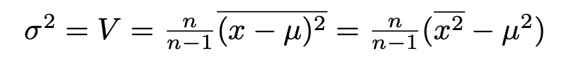
where the n/(n-1) factor, Bessel’s correction, just compensates for the fact that the squared standard deviation or variance of a sample is a biassed estimator of that of the parent. We know how to calculate the mean safely, and we can calculate the mean square in the same way. However we then hit another problem if, as often happens, the mean is large compared to the standard deviation.

Suppose what we’ve got is approximately Gaussian (or normal, if you prefer) with a mean of 100 and a standard deviation of 1. Then the calculation in the right hand bracket will look like

10001 – 10000

which gives the correct value of 1. However we’ve put two five-digit numbers into the sum and got a single digit out. If we were working to 5 significant figures, we’re now only working to 1. If the mean were ~1000 rather than ~100 we’d lose two more. There’s a significant loss of precision here.

If the first rule is not to add two numbers of different magnitude, the second is not to subtract two numbers of similar magnitude. Following these rules is hard because an expression like x+y can be an addition or a subtraction depending on the signs of x and y.

This danger can be avoided by doing the calculation in two passes. On the first pass you calculate the mean, as before. On the second pass you calculate the mean of (x-μ)2 where the differences are sensible, of order of the standard deviation. If your data is in an array this is pretty easy to do, but if it’s being read from a file you have to close and re-open it – and if the values are coming from an online data acquisition system it’s not possible.

And there is a solution. It’s called the Welford Online Algorithm and the code can be written as a simple extension of the running-mean program above

 // Welford's algorithm
 
float mean=x[0];
float V=0;
for(int j=1;j<n;j++){
     float oldmean=mean;
     mean += (x[j]-mean)/(j+1);
     V += ((x[i]- mean)(x[i]-oldmean) - V)/j
     } 
float sigma=sqrt(V);

The subtractions and the additions are safe. The use of both the old and new values for the mean accounts algebraically, as Welford showed, for the change that the mean makes to the overall variance. The only differences from our original running average program are the need to keep track of both old and new values, and initially defining the mean as the first element (zero), so the loop starts at j=1, avoiding division by zero: the variance estimate from a single value is meaningless. (It might be good to add a check that n>1 to make it generally safe).

I had suspected such an algorithm should exist but, after searching for years, I only found it recently (thanks to Dr Manuel Schiller of Glasgow University). It’s beautiful and its useful and it deserves to be more widely known.

It is amazing how simple computation can have profound complexity once you start digging.

What’s wrong with Excel?

I just posted a tweet asking how best to dissuade a colleague from presenting results using Excel.

The post had a fair impact – many likes and retweets – but also a lot of people saying, in tones from puzzlement to indignation, that they saw nothing wrong with Excel and this tweet just showed intellectual snobbery on my part.

A proper answer to those 31 replies deserves more than the 280 character Twitter limit, so here it is.

First, this is not an anti-Microsoft thing. When I say “Excel” I include Apple’s Numbers and LibreOffice’s Calc. I mean any spreadsheet program, of which Excel is overwhelmingly the market leader. The brand name has become the generic term, as happened with Hoover and Xerox.

Secondly, there is nothing intrinsically wrong with Excel itself. It is really useful for some purposes. It has spread so widely because it meets a real need. But for many purposes, particularly in my own field (physics) it is, for reasons discussed below, usually the wrong tool.

The problem is that people who have been introduced to it at an early stage then use it because it’s familiar, rather than expending the effort and time to learn something new. They end up digging a trench with a teaspoon, because they know about teaspoons, whereas spades and shovels are new and unfamiliar. They invest lots of time and energy in digging with their teaspoon, and the longer they dig the harder it is to persuade them to change.

From the Apple Numbers standard example. It’s all about sales.

The first and obvious problem is that Excel is a tool for business. Excel tutorials and examples (such as that above) are full of sales, costs, overheads, clients and budgets. That’s where it came from, and why it’s so widely used. Although it deals with numbers, and thanks to the power of mathematics numbers can be used to count anything, the tools it provides to manipulate those numbers – the algebraic formulae the graphs and charts – are those that will be useful and appropriate for business.

That bias could be overcome, but there is a second and much bigger problem. Excel integrates the data and the analysis. You start with a file containing raw numbers. Working within that file you create a chart: you specify what data to plot and how to plot it (colours, axes and so forth). The basic data is embellished with calculations, plots, and text to make (given time and skill) a meaningful and informative graphic.

In the alternative approach (the spade or shovel of the earlier analogy) is to write a program (using R or Python or Matlab or Gnuplot or ROOT or one of the many other excellent languages) which takes the data file and makes the plots from it. The analysis is separated from the data.

Let’s see how this works and why the difference matters. As a neutral example, we’ll take the iris data used by Fisher and countless generations of statistics students. It’s readily available. Let’s suppose you want to plot the Sepal length against the Petal length for all the data. It’s very easy, using a spreadsheet or using a program

Using Apple Numbers (other spreadsheets will be similar) you download the iris data file, open it, and click on

  • Chart
  • Scatter-plot icon.
  • “Add Data”
  • Sepal Length column
  • Petal Length column

and get

In R (other languages will be similar) you read the data (if necessary) and then draw the desired plot

iris=read.csv("filename")
plot(iris$Sepal.Length, iris$Petal.length)

and get

Having looked at your plot, you decide to make it presentable by giving the axes sensible names, by plotting the data as solid red squares, by specifying the limits for x as 4 – 8 and for y as 0 – 7, and removing the ‘Petal length’ title.

Going back to the spreadsheet you click on:

  • The green tick by the ‘Legend’ box, to remove it
  • “Axis”
  • Axis-scale Min, and insert ‘4’ (the other limits are OK)
  • Tick ‘Axis title’
  • Where ‘Value Axis’ appears on the plot, over-write with “Sepal Length (cm)”
  • ‘Value Y’
  • Tick ‘Axis title’
  • Where ‘Value Axis’ appears, over-write with “Petal Length(cm)”
  • “Series”
  • Under ‘Data Symbols’ select the square
  • Click on the chart, then on one of the symbols
  • “Style”
  • ‘Fill Color’ – select a nice red
  • ‘Stroke Color’ – select the same red

In R you type the same function with some extra arguments

plot(iris$Sepal.Length,iris$Petal.Length,xlab="Sepal length (cm)", ylab="Petal length (cm)", xlim=c(4,8), ylim=c(0,7), col='red', pch=15)

So we’ve arrived at pretty much the same place by the two different routes – if you want to tweak the size of the symbols or the axis tick marks and grid lines, this can be done by more clicking (for the spreadsheet) or specifying more function arguments (for R). And for both methods the path has been pretty easy and straightforward, even for a beginner. Some features are not immediately intuitive (like the need to over-write the axis title on the plot, or that a solid square is plotting character 15), but help pages soon point the newbie to the answer.

The plots may be the same, but the means to get there are very different. The R formatting is all contained in the line

plot(iris$Sepal.Length,iris$Petal.Length,xlab="Sepal length (cm)", ylab="Petal length (cm)", xlim=c(4,8), ylim=c(0,7), col='red', pch=15)

whereas the spreadsheet uses over a dozen point/click/fill operations. Which are nice in themselves but make it harder to describe what you’ve done – that left hand column up above is much longer than the one on the right. And that was a specially prepared simple example. If you spend many minutes of artistic creativity improving your plot – changing scales, adding explanatory features, choosing a great colour scheme and nice fonts – you are highly unlikely to remember all the changes you made, to be able to describe them to someone else, or to repeat them yourself for a similar plot tomorrow. And the spreadsheet does not provide such a record, not in the same way the code does.

Now suppose you want to process the data and extract some numbers. As an example, imagine you want to find the mean of the petal width divided by the sepal width. (Don’t ask me why – I’m not a botanist).

  • Click on rightmost column header (“F”) and Add Column After.
  • Click in cell G2, type “=”, then click cell C2, type “/”, then cell E2, to get something like this

(notice how your “/” has been translated into the division-sign that you probably haven’t seen since primary school. But I’m letting my prejudice show…)

  • Click the green tick, then copy the cell to the clipboard by Edit-Copy or Ctrl-C or Command-C
  • Click on cell G3, then drag the mouse as far down the page as you can, then fill those cells by Edit-Paste or Ctrl-V or Command-V
  • Scroll down the page, and repeat until all 150 rows are filled
  • Add another column (this will be H)
  • Somewhere – say H19 – insert “=” then “average(“,click column G , and then “)”. Click the green arrow
  • Then, because it is never good just to show numbers, in H18 type “Mean width ratio”. You will need to widen the column to get it to fit

Add two lines to your code:

> ratio=iris$Petal.Width/iris$Sepal.Width
> print(paste("Mean width ratio",mean(ratio)))
[1] "Mean width ratio 0.411738307332676"

It’s now pretty clear that even for this simple calculation the program is a LOT simpler than the spreadsheet. It smoothly handles the creation of new variables, and mathematical operations. Again the program is a complete record of what you’ve done, that you can look at and (if necessary) discuss with others, whereas the contents of cell 19 are only revealed if you click on it.

As an awful warning of what can go wrong – you may have spotted that the program uses “mean” whereas the spreadsheet uses “average”. That’s a bit off (Statistics 101 tells us that the mode, the mean and the median are three different ‘averages’) but excusable. What is tricky is that if you type “mean(” into the cell, this gets autocorrected to “median(“. What then shows when you look at the spreadsheet is a number which is not obviously wrong. So if you’re careless/hurried and looking at your keyboard rather than the screen, you’re likely to introduce an error which is very hard to spot.

This difference in the way of thinking is brought out if/when you have more than one possible input dataset. For the program, you just change the name of the data file and re-run it. For the spreadsheet, you have to open up the new file and repeat all the click-operations that you used for the first one. Hopefully you can remember what they are – and if not, you can’t straightforwardly re-create them by examining the original spreadsheet.

So Excel can be used to draw nice plots and extract numbers from a dataset, particularly where finance is involved, but it is not appropriate

  • If you want to show someone else how you’ve made those plots
  • If you are not infallible and need to check your actions
  • If you want to be able to consider the steps of a multi-stage analysis
  • If you are going to run the same, or similar, analyses on other datasets

and as most physics data processing problems tick all of these boxes, you shouldn’t be using Excel for one.

The Lesson from the Prisoner’s Dilemma

This is a classic puzzle which, like all such, comes in the form of a story. Here is one version:


Alice and Bob are criminals. No question. They have been caught red-handed in a botched robbery of the Smalltown Store, and are now in jail awaiting trial.

The police have realised that Alice and Bob match the description of the pair who successfully robbed the Bigtown Bank last month. They really want to get a conviction for that, but with no evidence apart from the resemblance they need to get a confession.

So they say to Alice: “Look, you are going to get a 1 year sentence for the Smalltown Store job, no question. But if you co-operate with us by confessing that the two of you did the Bigtown Bank heist then we’ll let you go completely free. You can claim Bob was the ringleader and he’ll get a 10 year sentence.”

Alice thinks a moment and asks two questions.

“Are you making the same offer to Bob? What happens if we both confess?”

The police tell her that yes, they are making the same offer to both of them. And if both confess, they’ll get 6 years each.


OK, that’s the story. All that circumstantial detail is just to lead up to this decision table, which Alice is now looking at:

Bob
Confess Deny
Alice Confess 6+6 0+10
Deny 10+0 1+1

That’s the problem in a nutshell. Before we look at it there are maybe a few points to clear up

  • Alice and Bob are not an item. They are just business partners. Each is aiming to minimise their own jail term, and what happens to the other is irrelevant for them.
  • ‘Go free’ really does mean that – there are no vengeful families or gang members to bring retribution on an informer.
  • Whether they actually committed the Bigtown Bank job is completely irrelevant to the puzzle.

OK, let’s get back to Alice. She reasons as follows:

“I don’t know what Bob is going to do. Suppose he denies the bank job. Then I should confess, to reduce my sentence from 1 year to zero. But what if he confesses? In that case, I’d better confess too, to get 6 years rather than 10. Whichever choice Bob makes, the better option for me is to confess. So I’ll confess.”

Bob will, of course, reason the same way. If Alice denies, he should confess. If Alice confesses, he should confess. 0 is less than 1, and 6 is less than 10. Therefore he should confess.

The logic is irrefutable. But look at that table again. The prisoners have firmly chosen the top left box, and will both serve 6 years. That’s a terrible result! It’s not only the worst total sentence (12 years), its the next-to-worst individual sentence (6 years is better than 10, but much worse than 0 or 1). Clearly the bottom right is the box to go for. It’s the optimal joint result and the next-to-optimal individual result.

That is obvious to us because we look at the table as a whole. But Bob (or Alice) can only consider their slices through it and either slice leads to the Confess choice. To see it holistically one has to change the question from the Prisoner’s Dilemma to the Prisoners’ Dilemma. That’s only the movement of an apostrophe, but it’s a total readjustment of the viewpoint. A joint Bob+Alice entity, if the police put them in one room together for a couple of minutes (but they won’t), can take the obvious bottom-right 1+1 choice. Separate individual Bob or Alice units, no matter how rational, cannot do that.

This is what the philosophers call emergence. The whole is more than just the sum of its parts. A forest is more than a number of trees. An animal is more than a bunch of cells. It’s generally discussed in terms of complex large-N systems: what’s nice about the Prisoner’s Dilemma is that emergence appears with just N=2. There is a Bob+Alice entity which is more than Bob and Alice seperately, and makes different (and better) decisions.

There’s also a lesson for politics. It’s an illustration of the way that Mrs Thatcher was wrong: there is such a thing as society, and it is more than just all its individual members. Once you start looking for them, the world is full of examples where groups can do things that individuals can’t – not just from the “united we stand” bundle-of-sticks argument but because they give a different viewpoint.

  • I should stockpile lavatory paper in case there’s a shortage caused by people stockpiling lavatory paper.
  • When recruiting skilled workers it’s quicker and cheaper for me to poach yours rather than train my own.
  • My best fishing strategy is to catch all the fish in the pond, even though that leaves none for you, and none for me tomorrow.
  • If I get another cow that will always give me more milk, even though the common grazing we share is finite.

Following the last instance, economists call this “The tragedy of the commons”. It’s the point at which Adam Smith’s “invisible hand” fails.

This tells us something about democracy. A society or a nation is more than just the individuals that make it up. E pluribus unum means that something larger, more powerful and – dare one say it – better can emerge. So democracy is more than just arithmetical counting noses, democracy provides the means whereby men and women can speak with one voice as a distinct people. That’s the ideal, anyway, and – even if the form we’ve got is clunky and imperfect – some of us still try to believe in it.

Why can’t science journalists understand p-values?

X1T

The Xenon1T experiment has just announced a really interesting excess of events, which could be due to axions or some other new particle or effect. It’s a nice result from a difficult experiment and the research team deserve  a lucky break. Of course like any discovery it could be a rare statistical fluctuation which will go away when more data is taken. They quote the significance as 3.5 sigma, and we can actually follow this: they see 285 events where only 232 are expected: the surplus of 53 is just 3.5 times the standard deviation you would expect from Poisson statistics: 15.2 events, the square root of 232.

This is all fine. But the press accounts – as in, for example,   Scientific American, report this as “there’s about a 2 in 10,000 chance that random background radiation produced the signal”.  It’s nothing of the sort.

Yes, the probability of exceeding 3.5 sigma (known as the p-value) is actually 2.3 in 10,000. But that’s not the probability that the signal was produced by random background. It’s the probability that random background would produce the signal. Not the same thing at all.

a

What’s the difference? Well, if you buy a lottery ticket there is, according to Wikipedia, a 1 in 7,509,578 chance of winning a million pounds.  Fair enough.  But now you meet a millionaire and ask  “What is the chance they got that way through last week’s lottery?” it’s certainly not 1 in 7,509,578.

There are several paths to riches: inheritance, business and of course previous lottery winners who havn’t spent it all yet. The probability that some plutocrat got that way through a particular week’s lottery depends not just on  that 1 in 7,509,578 number but on  the number of people who buy lottery tickets, and the number of millionaires by  who made their pile by other means. (It’s then just given by Bayes’ theorem – I’ll spare you the formula.)  You can’t find the answer by just knowing p, you need all the others as well.

There is a 1 in 7 chance that your birthday this year falls on a Wednesday, but if today is Wednesday, the probability that it’s your birthday is not 1 in 7. Your local primary school teacher is probably a woman, but most women are not primary teachers. All crows are black, but not all black birds are crows. Everyday examples are all around. For instance – to pick an analogous  one – if you see strange shapes in the sky this could be due to either flying saucers or to unusual weather conditions. Even if a meteorologist calculates that such conditions are very very unusual, you’ll still come down in favour of the mundane explanation.

clouds So going back to the experiment,  the probability that random background would give a signal like this may be 1 in 20,000 but that’s not the probability that this signal was produced by  random background: that also depends on the probabilities we assign to the mundane random background or the exotic axion. Despite this 1 in 20,000 figure I very much doubt that you’d find a particle physicist outside the Xenon1T collaboration who’d give you as much as even odds on the axion theory turning out to be the right one. (Possibly also inside the collaboration, but it’s not polite to ask.)

This is a very common mistake – every announcement of an anomaly comes with its significance reported in terms of the number of sigma, which somebody helpfully translates into the equivalent p-value, which is then explained wrongly, with language like “the probability of the Standard Model being correct is only one in a million” instead of “the probability that the Standard Model would give a result this weird is only one in a million”.   When you’re communicating science then you  use non-technical language so people understand – but you should still get the facts right.


The Monty Hall Puzzle

There are many probability paradoxes, but the Monty Hall Puzzle is much the greatest of these, provoking more head scratching and bafflement than any other.

It is easy to state. Monty Hall hosted a TV quiz show “Let’s Make a Deal”, in which a contestant has to choose one of 3 doors: behind one of these is a sports car, whereas the other two both contain a goat. (Some discussions of the puzzle – and there are many – speak of ‘a large prize or smaller prizes’, but they can be dismissed as non-canonical; the goats are essential.) There is no other information, so the contestant has a 1 in 3 chance of guessing correctly. Let’s say, without loss of generality, that they pick door 1.

But Monty doesn’t open it straight away. Instead he opens one of the other 2 doors – let’s say it’s door 3 – and shows that it contains a goat. He then offers the contestant a chance to switch their choice from the original door 1 to door 2.

Should the contestant switch? Or stick? Or does it make no difference?

That’s the question. I suggest you think about it before reading on. What would you do?  Bear in mind that the pressure is on, you are in a spotlight with loud music building up tension, and Monty is insistent for an answer. Putting the contestant under pressure makes good television.

Several arguments are put forward – often vehemently

  1. You should switch: the odds were 1/3 that door 1 was the winner, and 2/3 that it was one of the other doors. You now know the car isn’t behind door 3, so all that 2/3 collapses onto door 2. Switching doubles your chance from 1/3  to 2/3.
  2. There’s no point in switching: all you actually know, discarding the theatricality, is that the car is either behind door 1 or door 2, so the odds are equal.
  3. But you should switch! Suppose there were 100 doors rather than 3. You choose one, and Monty opens 98 others, revealing 98 goats, leaving just one of the non-chosen doors unopened.  You’d surely want to switch to that door he’s so carefully avoided opening.

Thought about it?  OK, the answer is that there is no answer. You don’t yet have enough information to make the decision, as you need to know Monty’s strategy. Maybe he wants you to lose, and only offers you the chance to switch because you’ve chosen the winning door. Or maybe he’s kind and is offering because you’ve chosen the wrong door. (There’s a pragmatic let-out which says that if you don’t know whether to switch or stick you might as well switch, as it can’t do any harm – we can close that bolthole by supposing that Monty will charge you a small amount, $10 or so, to change your mind.)

OK, let’s suppose we know the rules and they are

  1. Monty always opens another door.
  2. He always opens a door with a goat and offers the chance to switch. If both non-chosen doors contain goats he chooses either at random.

Now we have enough information. We can analyse this using frequentist probability, which is what we learnt at school.

 Suppose we did this 1800 times ( a nice large number with lots of useful factors). Then the car would be behind each door 600 times. Alright, not exactly 600 because of the randomness of the process, but the law of large numbers ensures it will be close.

A door is then chosen – this is also random so in each of the 3 x 600 cases door 1 will be chosen in only 3 x 200 times. The other cases can now be discarded as we know they didn’t happen. 

For the 200 cases where the car is behind door 1,  Monty will open door 2 and door 3 100 times each. We know he didn’t open door 2, so only 100 cases survive. But all 200 cases with the car behind door 2 survive, as for them he is sure open door 3. When the car is behind door 3 he is never going to open it. So of the original 1800 instances, door 1 is chosen and door 3 is opened in 300 cases, of which 200 involve a winning door 2 and only 100 have door 1 as the winner. Within this sample the odds are 2:1 in favour of door 2. You should switch!

You can also show show this using Bayes’ theorem. Maybe I’ll write about Bayes’ theorem another time.  For the moment, let’s just accept that when you have data, prior probabilities are multiplied by the likelihood of getting that data, subject to overall normalisation.

The initial probability is 1/3 for each door.

P1=P2=P3=1/3

The ‘data’ is that Monty chose to open door 3.  If the winner is door  2, he will certainly open door 3. If it is door 3, he will not open it. If it is door 1, there is a 50% chance of picking door 3 (and 50% for door 2). So the likelihoods are   1/ 2 , 1 and 0 respectively, and after normalisation

P1‘ = 1/ 3         P2‘ = 2/ 3         P3‘=0

So switch! It doubles your chances. 

If you think that’s all obvious and are feeling pretty smug, let’s try a slightly different version of the rules:

  1. Monty always opens another door.
  2. He does this at random. If it reveals a car, he says ‘Tough.” If it contains a goat, he offers a switch.

The frequentist analysis is similar: starting with 1800 cases, if door 1 is chosen then that leaves 600, with 200 for each door being the winner. Now he opens doors 2 and 3 with equal probability, whatever the winning door may be. If it’s door 1, 100 survive as before. If it’s door 2, this time only 100 survive, and in the other hundred he opens door 2 to show a car. For door 3 there are no survivors as he either reveals a goat behind door 2 or a car behind door 3, neither of which has happened. So in this scenario there are 200 survivors, 100 each for doors 1 and 2. The odds are even and there is no point in switching.

Using Bayes’ theorem gives (of course) the same result. The prior probabilities are still all  1/ 3.  The likelihood for Monty to pick door 3 and reveal a goat is  1/ 2 for both door 1 and door 2 concealing a car, and zero for door 3.  Normalising

P1‘ = 1/ 2         P2‘ = 1/ 2         P3‘=0

and theres no point in switching.

So a slight change in the rules switches the result. The arguments 1 to 3 are all suspect.  Even the 3rd argument (which I personally find pretty convincing) is not valid for the second set of rules. If Monty opens 98 doors at random to reveal 98 goats this does not make it any more likely that the 99th possibility is the winner.

If you don’t believe that – or any of the other results – then the only cure is to write a simulation program in the language of your choice. This will only take a few lines, and seeing the results will convince you where mathematical logic can’t.

So the moral is to be very wary of common sense and “intuition” when dealing with probabilities, and to trust only in the results of the calculations. Thank you, Monty!