Why can’t science journalists understand p-values?

X1T

The Xenon1T experiment has just announced a really interesting excess of events, which could be due to axions or some other new particle or effect. It’s a nice result from a difficult experiment and the research team deserve  a lucky break. Of course like any discovery it could be a rare statistical fluctuation which will go away when more data is taken. They quote the significance as 3.5 sigma, and we can actually follow this: they see 285 events where only 232 are expected: the surplus of 53 is just 3.5 times the standard deviation you would expect from Poisson statistics: 15.2 events, the square root of 232.

This is all fine. But the press accounts – as in, for example,   Scientific American, report this as “there’s about a 2 in 10,000 chance that random background radiation produced the signal”.  It’s nothing of the sort.

Yes, the probability of exceeding 3.5 sigma (known as the p-value) is actually 2.3 in 10,000. But that’s not the probability that the signal was produced by random background. It’s the probability that random background would produce the signal. Not the same thing at all.

a

What’s the difference? Well, if you buy a lottery ticket there is, according to Wikipedia, a 1 in 7,509,578 chance of winning a million pounds.  Fair enough.  But now you meet a millionaire and ask  “What is the chance they got that way through last week’s lottery?” it’s certainly not 1 in 7,509,578.

There are several paths to riches: inheritance, business and of course previous lottery winners who havn’t spent it all yet. The probability that some plutocrat got that way through a particular week’s lottery depends not just on  that 1 in 7,509,578 number but on  the number of people who buy lottery tickets, and the number of millionaires by  who made their pile by other means. (It’s then just given by Bayes’ theorem – I’ll spare you the formula.)  You can’t find the answer by just knowing p, you need all the others as well.

There is a 1 in 7 chance that your birthday this year falls on a Wednesday, but if today is Wednesday, the probability that it’s your birthday is not 1 in 7. Your local primary school teacher is probably a woman, but most women are not primary teachers. All crows are black, but not all black birds are crows. Everyday examples are all around. For instance – to pick an analogous  one – if you see strange shapes in the sky this could be due to either flying saucers or to unusual weather conditions. Even if a meteorologist calculates that such conditions are very very unusual, you’ll still come down in favour of the mundane explanation.

clouds So going back to the experiment,  the probability that random background would give a signal like this may be 1 in 20,000 but that’s not the probability that this signal was produced by  random background: that also depends on the probabilities we assign to the mundane random background or the exotic axion. Despite this 1 in 20,000 figure I very much doubt that you’d find a particle physicist outside the Xenon1T collaboration who’d give you as much as even odds on the axion theory turning out to be the right one. (Possibly also inside the collaboration, but it’s not polite to ask.)

This is a very common mistake – every announcement of an anomaly comes with its significance reported in terms of the number of sigma, which somebody helpfully translates into the equivalent p-value, which is then explained wrongly, with language like “the probability of the Standard Model being correct is only one in a million” instead of “the probability that the Standard Model would give a result this weird is only one in a million”.   When you’re communicating science then you  use non-technical language so people understand – but you should still get the facts right.


Tips for speakers#2: Beware of the second slide

Screenshot 2020-03-21 at 14.21.03

In a million and one grad student talks the second slide looks like this: the table-of-contents or the  outline-of-the-talk. It may be a bit more colourful, with banners and logos and exciting pictures, but it’s basically the same, and the speaker will repeat the traditional phrases “After an introduction and a survey of the literature, I’ll describe the methodology we used…”

By this stage, one minute into the talk, the members of the audience are all thinking “Here’s another grad student talk like a million others… so predictable. ” and their attention will wander to their unanswered emails, or their plans for dinner, or an attractively-filled T shirt two rows in front, and the poor speaker has got to work really hard to get them back.

Do you need a contents slide at all?  It’s not compulsory.  Even though some presentation packages provide it almost by default, with sections and subsections, you don’t have to have one.  Before you include it you should weigh up the reasons for and against.

Against:

  • It cuts into your time allocation.
  • It disrupts the flow of the talk as, by definition, it stands outside the narrative.
  • It will tend to shift the focus onto you as the speaker rather than on the material

On the other hand:

  • It can give structure to an otherwise amorphous talk
  • It can help the audience keep track of a complicated sequence of ideas

So its inclusion or exclusion depends on the talk length, the nature of  the material, the links between you and your audience, and your personal style. In a 10 minute conference oral where you’re developing one idea it’s almost certainly not wanted. In a one hour seminar covering disparate but linked topics it could be really useful.  If you’re going to include an outline, that should be a conscious decision, not just something you feel you ought to do.

If you do decide to include one, then make it work for you. Refer back to it during the talk, showing the audience where they’ve got to on the map you set out at the start. (There are some Beamer  themes that do this automatically – Berkeley is a standard.  UpSlide does it for PowerPoint. But it’s easy to do it by hand.) If you’re including an outline then make full use of it.  

Screenshot 2020-03-21 at 16.28.27The final point is: if you’ve decided to include a table of contents then customize it. Make it your own and unique so that it’s not just the same as every other grad student talk. Here’s a revised version of that original outline slide (with some invented details). It’s the same slide: the first bullet is the introduction, the second is the literature search, and so on. But don’t call them that. Fill in your details  in the generic slots, and that will keep the audience engaged and attentive and get them into your world and your language from the start. 

Probability and job applications

In preparing a recent talk on probability for physics grad students – it’s here if you’re interested – I thought up a rather nice example to bring out a key feature of frequentist probability. I decided not to include it, as the talk was already pretty heavy, but it seemed too good an illustration to throw away. So here it is.

Suppose you’ve applied for a job. You make the short list and are summoned for interview. You learn that you’re one of 5 candidates.

So you tell yourself – and perhaps your partner – not to get too hopeful.  There’s only a 20% probability of your getting the job.

But that’s wrong.

That 20% number is a joint property of yourself and what statisticians call the collective, or the ensemble.  Yes, you are one of a collective of 5 candidates, but those candidates are not all the same.

Let me tell you – from my experience of many job interviews, good and bad, on both sides of the table, about those 5 candidates .

hiring-1977803_1280

One candidate will not turn up for the interview. Their car will break down, or their flight will be cancelled, or they will be put in Covid-19 quarantine. Whether their subconscious really doesn’t want them to take this job, or they have a guardian angel who knows it would destroy them, or another candidate is sabotaging them, or they’re just plain unlucky, they don’t show.   There’s always one.

A second candidate will be hopeless. They will have submitted a very carefully prepared CV and application letter that perfectly match everything in the job specification, bouncing back all the buzz-words and ticking all the boxes so that HR says they can’t not be shortlisted. But at the interview they turn out to be unable to do anything except repeat how they satisfy all the requirements, they’ll show no signs of real interest in the work of the job apart from the fact that they desperately want it.

The third candidate will be grim. Appointable, but only just above threshold. The members of the panel who are actually going to work with them are thinking about how they’re going to have to simplify tasks and provide support and backup, and how they really were hoping for someone better than this.

Candidate four is OK.  Someone who understands the real job, not just the job spec in  the advert, and who has some original (though perhaps impractical) ideas. They will make a success of the job and though there will be occasional rough patches they won’t need continual support.

Candidate five is a star. Really impressive qualification and experience on paper, glowing references, and giving a superb interview performance, answering questions with ease and enthusiasm and using them to say more. They will certainly get offered the job – at which point they will ask for a delay, and it will become clear that they’re also applying for a much better job at a superior institution, and that they don’t really want this one which is only an insurance in case they don’t get their top choice.

So there are the five. (Incidentally, they are distributed evenly between genders, backgrounds and ethnicities). Don’t tell yourself your chance is 20%. That’s true only in the sense that your chance of being male (as opposed to female) is 50%.  Which it is, as far as I’m concerned, but certainly not as far as you’re concerned.

Instead ask yourself – which of the five candidates are you?

(If you don’t know, then you’re candidate #3)


Tips for speakers #1: don’t thank the audience for their attention

One problem anyone faces in putting any sort of talk together is how to finish.  And a depressingly large number of speakers do so with a slide like this

Screenshot 2019-06-15 at 15.27.05

This way of ending a talk came originally, I think, from Japan. And unless you are Japanese you should never use it. A Japanese speaker has centuries of proud samurai tradition behind them, and when they say ” thank you for your attention” what they mean is

Screenshot 2019-06-15 at 15.22.15

If you are not Japanese this does not work. Instead the message conveyed is

Screenshot 2019-06-15 at 15.24.52

Which is not a good way to finish.

And this throws away a golden opportunity.  The end of the talk is the point at which you really have the attention of the audience. This may not be for the best of reasons – perhaps they want to hear the next speaker, or to go off for much-needed coffee, but when you put your conclusions slide up your listeners’ brains move up a gear. They look up from the email on their laptops and wonder what’s next. So your final message is the one with the best chance of being remembered.

Give them the pitch that you hope they’ll take away with them.

“So we have the best results yet on ….”

“So we have the prospect of getting the best results on … in time for next year’s conference”

“There are going to be many applications of this technique”

“We understand the whole process of … a lot better”

Whatever’s appropriate.  Be positive and upbeat and, even if they’ve been asleep for the past 20 minutes,  they will go away with a good feeling about your work, your talk, and your ability as a speaker.


(See what I just did??)


LHCb clocks up 8 Inverse femtobarns

The LHCb experiment has just announced that it’s accumulated 8 inverse femtobarns of data. The screen shows the result and the ongoing totals.

It’s obviously a cause for celebration, but maybe this is an opportunity to explain the rather obscure ‘inverse femtobarn’ unit.

Let’s start with the barn. It’s a unit of area. 10 -28 square metres, so rather small. It was invented by the nuclear physicists to describe the effective target-size corresponding to a particular nuclear reaction. When you fire beam particles at target particles then all sorts of things can happen, with probabilities predicted by complicated quantum mechanical calculations,  but those probabilities can be considered as if each reaction had its own area on the target nucleus: the bigger the area the more likely the reaction. It’s not literally true, of course, but the dimensions are right and you can use it as a model if you don’t push it too far.  Nuclear cross sections, usually called σ, are typically  few barns, or fractions of a barn, so it’s a handy unit.

No, it’s not named after some Professor Barn – it’s probably linked to expressions like “Couldn’t hit the broad side of a barn” or even “Couldn’t hit a barn door with a banjo!”

Particle physicists took this over, though our cross sections were typically smaller – millibarns (10-3 barns) for strong interaction processes, microbarns (10-6) and nanobarns (10-9) for electromagnetic processes such as were measured at PETRA and LEP.  Beyond that lie picobarns (10-12) and femtobarns(10-15).   Only the neutrino physicists stuck with m2 or cm2 as their cross sections are so small that even using attobarns can’t give you a sensible number. So a femtobarn is just a cross section or area, 10-43 , square metres.

In a colliding beam storage ring like the LHC, Luminosity measures the useful collision rate, how many particles are in the beams, how tightly the beams have been focussed and how well they are aligned when they collide.  The event rate is the produce of the cross section and the luminosity, R=Lσ so luminosity is what accelerator designers set out to deliver. Integrated luminosity is just  luminosity integrated over time, and ∫L dt = N/σ, as  the integrated rate is just the total number of events,∫R dt = N

So there we have it.  An integrated luminosity of 8 inverse femtobarns (written 8 fb-1  or 8 (1/fb) ) means that for a cross section as tiny as 8 fb, one would expect to see, on average,  8 events. 8 is a measurable number – though that depends on backgrounds –  but what this is saying is that we can detect (if they’re there) rare processes that have cross sections of order 1 fb.   That’s the sort of number that many Beyond-the-Standard-Model theories come up with. It’s pushing back the frontier.

If you look at the screen you can see the recorded number as 8000 pb-1. Yes, an inverse femtobarn is bigger than an inverse picobarn. Which is obvious if you think about it, but disconcerting until you do.

Another point to take from the picture is that the LHC accelerator actually delivered more. 8769.76 pb-1 were delivered to get the 8000 taken. The loss is inevitable due to time lost to ramping voltages,  detector calibration and the overall efficiency of over 90% is pretty good.

So it’s a landmark.  But these BSM processes havn’t shown up yet and until they do we need to keep taking data – and increase the luminosity. Both the LHCb  detector and the LHC accelerator are working hard to achieve this – both are needed, as the detector has to be able to handle the increased data it’s being given. So we’ve passed a milestone, but there’s still a long and exciting road ahead.

Why is the sky blue?

This is a stock ‘Ask the physicist’ question and most physicists think they know the answer. Actually, they only know half the story.

The usual response is “Rayleigh Scattering”.  On further probing they will remember, or look up, a formula like

for the intensity of light  scattered at an angle θ by molecules of polarisability α  a distance R away.

The sky is blue

The key point to this formula is that  the intensity is proportional to the inverse 4th power of the wavelength. Light’s oscillating electric field pushes all the electrons in a molecule one way and all the nuclei the other, so the molecule (presumably Nitrogen or Oxygen in the stratosphere) responds like any simple harmonic oscillator to a forced oscillation well below its resonant frequency.  These oscillating charges act as secondary radiators of EM waves, and higher frequencies radiate more.  Visible light varies in frequency by about a factor of 2 over the spectrum  (actually a bit less but 2 will do – we speak of the `octave’ of visible EM radiation) so violet light is scattered 16 times as much as red light.  So when we look at the sky we see light from the sun that’s been scattered by molecules,  and it’s dominated by higher frequency / short wavelengths so it has  a blue colour – not completely violet as there is still some longer wavelength light presen

This also explains why light from the sun  at sunset (and sunrise),  which travels a long way through the atmosphere to get to us, appears redder, having lost its short wavelength component to provide a blue sky for those living to the west (or east) of where we are.  It also predicts and explains the polarisation of the scattered blue light: there are dramatic effects to be seen with a pair of polarised sunglasses, but this post’s quite long enough without going into details of them.

Most explanations stop there. This is just as well, because a bit more thought reveals problems. Why don’t light rays show this behaviour at ground level? Why don’t they scatter in solids and liquids, in glass and water? There are many more molecules to do the scattering, after all, but we don’t see any blue light coming out sideways from a light beam going through a glass block or a glass of water.

The reason appears when we consider scattering by several molecules. They are excited by the same EM wave and all start oscillating, the oscillations are secondary sources of EM radiation which could be perceived by an observer – except that they are, in general, out of phase.  The light from source to molecule to observer takes different optical paths for each molecule, and when you add them all together they will (apart from statistical variations which are insignificant) sum to zero. To put it another way, when you shine a light beam through a piece of glass and look at it from the side, you perceive different induced dipoles, but half will point up and half will point down, and there is no net effect.   The random phase factors only cancel if you look directly along or against the direction of the beam – against the beam the secondary sources combine to give a reflected ray, along the beam their combined effect  is out of phase with the original ray and their sum slips in phase – making the light beam slow down.


light scattered by different molecules is out of phase and sums to zero

So we’re stuck.  One molecule is not enough to turn the sky blue, you need many. But many molecules co-operate in such a way that there is no side scattering. Dust was once suggested as the reason but dust is only present in exceptional circumstances like after volcano eruptions.

The only way to do it would be if the molecules grouped together in clusters.   Clusters small compared to the wavelength of visible photons, but separated by distances large compared to their coherence length. Why would they ever do that?

But they do. Molecules in a gas – unlike those in a solid or liquid –  are scattered in random positions and form clusters by sheer statistical variation.  This clustering is enhanced by the attractive forces between molecules – the same forces that makes them condense into a liquid at higher pressures / lower temperatures.  So the fluctuations in density in the stratosphere are considerable; their size is small and their separation is large, and it’s these fluctuations in molecular density that give us the bright blue sky.

Molecules in a gas

The figure shows (very schematically) how this happens. In the first plot the density is very low and the few molecules are widely separated.  In the second the density is higher and even though the distribution shown here is random, clusters emerge due to statistical fluctuations. In the third plot these clusters are enhanced by attraction between the molecules. In the final plot the density is so high they form a solid (or liquid).

This puzzle was not solved by Rayleigh but by – yet again – Albert Einstein.  In 1910 he explained (Annalen der Physik 33 1275 (1910)) the size and nature of the density fluctuations in a gas, and showed how the theory explained the phenomenon of critical opalescence, when gases turn milky-white at the critical point, and that the sky was an example of this. It dosn’t even count as one of his ‘great’ papers – though it does follow on from his 1905 annus mirabilis paper on Brownian motion. He showed that our blue sky comes from light scattering not just off molecules, but off fluctuations in the molecular density.

So if anyone ever asks you why the sky is blue, be sure to give them the full story.

The Lorentz Transformation – a minimal proof

Lorentz
Einstein

You can find many ways in the textbooks to derive the Lorentz Transformation, starting from Einstein’s famous two postulates: that the laws of physics are the same in all inertial frames, and that the speed of light is a constant. You can do it in one big chunk, or by starting with length contraction and time dilation.

What I want to do here is show a proof which requires only one, surprisingly minimal, assumption, and  which relegates ‘light’ to its proper place as a subsidiary phenomenon. This is the opposite of the order which is usually taught, so this is not the sort of proof  you get in Relativity101, but after you’ve learnt and are happy with the standard proofs, I think you’ll appreciate this one.

We make some basic assumptions – as indeed we do in a conventional proof, though they’re not usually spelt out.  Events occur in continuous time t and continuous space r, though for simplicity we’ll just consider one space dimension x. Space and time are isotropic and homogeneous – there are no special times or places. We can plot events in space-time diagrams, where the t axis is calibrated using repeated identical processes like the swing of a pendulum or the vibrations of a crystal, and the x axis is calibrated using stationary identical rods.

Events cause, and are caused by, other events. For a pair of events A and B it could be that A→BA has a (possible) effect on B, or that B→A, B has a (possible) effect on A. In the first case we say that A lies in the past of B, and B is in the future of A. In the second case it’s the other way round. We dismiss the possibility that both A→B and B→A, as that leads to paradoxes of the killing-your-grandfather variety. But what about the possibility that neither A→B nor B→A: that there can be pairs of events for which neither can influence the other?

There’s not an obvious answer. If you were designing a universe you could insist that any pair of events must have a causal connection one way or the other, or you could allow the equivalent of the ‘Don’t know’ box. The choice is not forced on us by logic. But let’s suppose that we do live in a universe where this directed link between events is optional rather than compulsory:

There are pairs of events which are not causally connected.

I promised you a single assumption: there it is.  Now let’s build on it.

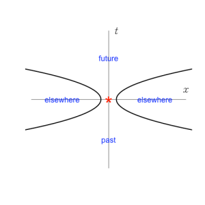
For any event there must be some events which are not causally connected. The assumption says this is for true for some events, but all events must be similar (as space and time are homogeneous) , so this is true in general.  So we can drawa  space-time diagram showing the events  that are  past, future, and elsewhere for an event at the origin.

Events lie in definite regions

Causality is transitive: if A→B and B→ C then A→ C, as A can influence C through B. That means that  at any particular point x, events that are in A‘ s past must be followed by elsewhere events and then future events. They can’t be mixed up.  The events occur in defined regions


The Elsewhere region extends to the origin

Even at small distances there must be elsewhere events – if there were some minimum distance from A, Δ, within which all events were either past or future,  and B is the event at Δ on the division between past and future, then all events within 2Δ of A must be in the past and future, and so on for 3,4,5….


The Elsewhere region is a simple wedge

The lines separating the past, elsewhere and future regions must be straight lines going through the origin. For any point B on the future light cone of A, the gradient of the line separating B‘ s elsewhere and future must have the same gradient as the light cone for A at x=0. But the future light cone of B defines the future light cone of A. So the gradient must be constant all the way. (The same applies for the past light cone, and symmetry requires that the gradient have the same magnitude.)

So to re-cap: first we establish that there are elsewhere events, then that they lie in regions, then that these regions go all the way to the origin, and finally that the shape of the elsewhere region is a simple double wedge. (It’s called a ‘light cone’ as you can imagine extending the picture to two space dimensions by rotating these 2D pictures about the vertical axis, but you probably knew that already.)

Out of this picture a number emerges: the gradient of the line dividing the elsewhere region from the future (or the past). We have no way of knowing what its value is – only that it is finite. It describes the speed of the fastest possible causal signal and we will, of course, denote it by c. It can be viewed as a fundamental property of the universe, or as a way of relating time measurement units to space ones.

Now we’re on more familiar ground. If an event that we denote by (x,t) is observed by someone in a different inertial frame moving at some constant speed relative to the first, they will ascribe different numbers (x’,t’). What is the transformation (x,t)→(x’,t’)?

  1. Let’s assume that zeros are adjusted so that (0,0) is just (0,0). That’s trivial.
  2. We require that vector equations remain true: if (xA,tA)=(xB,tB)+(xC,tC) then  (x’A,t’A)=(x’B,t’B)+(x’C,t’C). That limits us to linear transformations x’=Ax+Bt; t’=Cx+Dt. So the transformation is completely described by 4 parameters A,B,C and D.
  3. The inverse transform  (x’,t’) to (x,t) must be the same, except that the direction of the speed has changed. That’s the equivalent of changing the sign of x or t. So x=Ax’-Bt’; t=-Cx’+Dt’.   The transformation to the new frame and back again must take us exactly back to what we started with, i.e.  A(Ax+Bt)-B(Cx+Dt)=x.  From which we must have A=D and A2-BC=1. The four parameters are reduced to two.
  4. Finally we impose the requirement that the new co-ordinates (x’,t’) must lie in the same sector (past, present, or elsewhere) as the old. In particular, if x=ct then x’=ct’. That means Act+Bt=c(Cct+Dt) and using A=D from the previous paragraph, this shows B=c2C. The two parameters are reduced to one. This is most neatly expressed by introducing v=-B/A, as then A2-BC=1 gives our old friend A=1/√(1-v2/c2) and substituting A, B, C and D gives the familiar form of the Lorentz transformations.

    The Lorentz Transformation

Inspecting these shows that v, which we introduced as a parameter, describes the motion of the point x’=0, the origin of the primed frame, in the original frame, i.e. the speed of one frame with respect to the other.

A bit of algebra shows that the ‘interval’ of an event is the same: x2-c2t2=x’2-c2t’2. Which is neat, showing that the points lie on a hyperbola of which the light-cone crossed-lines is the limiting case, so they cannot move between sectors . But we didn’t have to assume that the interval is unchanged, only that an interval of zero remains zero.

So the Lorentz Transformation springs from the basic causal structure of space-time, assuming that not all events are causally connected one way or the other, with c the speed of the fastest causal signal, whatever that happens to be. Length contraction and time dilation follow from this. Then you discover that if you have Coulomb’s Law type electrostatics the Lorentz Transformations give you magnetism and Maxwell’s Equations emerge. These have wavelike solutions with wave velocity  c. 

In terms of logical argument, the causal structure of the universe just happens to include the possibility that 2 events cannot affect one another in either way. This fundamental property leads to relativity and the Lorentz Transformation,  which leads to electromagnetism, which then leads to EM waves and light, even though historically and pedagogically the sequence is presented the other way round.

The collapse of the wave function, and two sorts of time

Suppose a star emits a photon. Its wave function spreads over space, perhaps over light years.

On a far planet, a poet is looking at the night sky: if they  see that photon they will be inspired to write a great poem. Meanwhile at the other edge of the galaxy there is a pig, also, for its own porcine reasons, gazing skywards, and the photon wave function also passes through its retina. The pig may see the photon or the poet may see the photon. (Or, of course, it may be seen by neither.)  But it absolutely cannot be seen by both of them. If the photon materialises in an eyeball of one, it cannot do so in an eyeball of the other.  The wave function collapses, instantaneously and simultaneously across all space.

This rings alarm bells. The Theory of Relativity tells us loud and clear that ‘simultaneity’ is a dirty word, but it really does apply here. The arrival of the photon wave function at the pig and the poet may be simultaneous in the picture above, but there will be reference frames in which it arrives at the pig before the poet, and frames where the poet comes before the pig. Whatever frame you’re working in, the wave function collapse is simultaneous everywhere in that frame.

It’s the truly spooky bit of quantum mechanics that really nobody understands. An object – be it a photon, an electron, an atom, or a cat – has a wave function, and we can study the behaviour of that wave function by solving complicated differential equations. Then a measurement is made of some property, and the wave function changes randomly but instantly into a state where that property is defined. If the wave function is ‘real’ it defies relativity. If it is not ‘real’ then what is?

Most physicists solve this puzzle by ignoring it – the so-called ‘shut up and calculate’ school. I’m not going to explain the puzzle here – nobody can. What I do want to do is show that it is not really new, but linked to an older one.

Let’s introduce a logical formalism for discussing the collapse of the wave function in an ordered and well-defined way.  This was done by John von Neumann in his “Mathematical Foundations of Quantum Mechanics”, (Springer 1932, English translation by R T Beyer, Princeton, 1955) and what follows is his development, with modernised notation.

We need to introduce a neat concept called the density matrix.  This combines the two sorts of uncertainty that we have to deal with: quantum uncertainty and the established uncertainty of statistics and thermodynamics.

First, from quantum mechanics we take the idea of a basis set of states |i>, which are eigenstates of some measurement operator  (so Â |i> = ai|i>). In what follows I’ll use as an example the simple case where there are just two states describing the spin of an electron as up |↑> or down |↓>;  they could also be the states |x> of delta functions at particular positions, or the pure sine wave states |p> that have definite wavelength and thus definite momentum.

Secondly, from Statistical Mechanics we take the idea of a large ensemble of N states |ν>, which are the actual states of many systems in equilibrium with one another.  The  |ν> states are (in general) not the same as the |i> states but they can be written in terms of them: |ν> = Σi <i|ν>  |i>, because the |i> states are a basis set. <i|ν>  is a number, the i-component of the ν state in the ensemble.

Right, that’s the apparatus in place. The density matrix is just the average over the ensemble of the Cartesian product of the components

ρij=(1/N) Σν <i|ν> <ν|j>

What can you do with it? Well the diagonal elements ρii correspond to the average over the ensemble of | <ν|i> |2, which, according to the Born interpretation, is the probability of finding state |ν> in state |i> if you measure it with  . It tells us the probability of getting the result ai where the probability includes both the quantum uncertainty and the statistical uncertainty from the ensemble.

Density matrix for an up/down mixture

Let’s take an example.  If we take an ensemble of many electrons of which half are spin up and half are spin down then the matrix has 1/2  on each diagonal element and the off-diagonals are zero, because each    |ν> is either up or down, so the product of  <ν|> and <ν|↓> is always zero.  The diagonal tells us that if you pick an electron at random from the ensemble, there’s a 50% chance each for it being spin up or spin down.

Now let’s get a bit less trivial. We’ll take a sample of spin-down electrons, all the same this time,  and then rotate them 90 degrees about the y axis, so they point in the +x direction.

Rotating a spinor from down to sideways
Density matrix for electrons pointing sideways, along the x axis

These states give the density matrix which has the same diagonal elements as the last one, but non-zero off-diagonal elements. The diagonal elements tell us that there is, again, a 50:50 chance of detecting the electron in an up or down state, though this time it’s because of quantum uncertainty.

If the diagonal elements give the probabilities, you might wonder whether there’s any point to the off-diagonal elements. But they do play a part. Suppose that, for both examples, we rotate the spins buy another 90 degrees before we measure them.  Under a rotation R the density matrix becomes  ρ’=RρR. A bit of  matrix arithmetic shows the matrix for the first example is unchanged, on the second example, the sideways states, is

which is obvious, with hindsight. The second rotation converts the spin direction from the x to the z axis,  so they will always be in the spin up state if you measure them, whereas for the first example the result is still 50:50 unpredictable.

So the density matrix encompasses quantum uncertainties, which may become certain if you ask a different question, and statistical uncertainties which cannot.  Diagonal elements give probabilities and off-diagonal elements contain information on the degree of quantum coherence. If you want to know more about it, try Feynman’s textbook  “Statistical Mechanics: a set of lectures” (CRC press, 1998).

As time goes by the states will evolve, and the evolution of the density matrix has the apparently simple form ρ’=e-iHt/ℏ ρ eiHt/ℏ. I say ‘apparently simple’ because H, which is being exponentiated, is a matrix. But this is standard quantum mechanics and the techniques exist to handle it. The |i> wave functions  oscillate at their characteristic frequencies.

But the matrix can also describe the effect of a measurement of the quantity corresponding to the operator Â. The measurement asks of each state |ν > which of the |i> basis states it belongs to: if it is in one of those states it stays in it, if it is in a superposition then it will drop into one of the|i>, the probability for each being   |<i|ν >|2.  So the density matrix becomes ρ’ij= δij ρij. The diagonal elements are preserved, and all the off-diagonal elements vanish, as each member of the ensemble is now in a definite basis state.

To say ‘a measurement zeroes all the off-diagonal terms of the density matrix’ expresses the ‘collapse of the wave function’ correctly and completely, but in a smooth and non-sensational way.

These two equations,  ρ’=e-iHt/ℏ ρ eiHt/ℏ and ρ’ij= δij ρij, both describe how a system changes with time. They are different because the ‘time’ is different.

It is often (unkindly) said that there are as many philosophies of time as there are philosophers of time, but if you ignore the weirdest ones and brush over the details there are basically two.

In first concept, the time of Parmenides, Plato, Newton, Einstein and Hawking,  sometimes called ‘Being Time‘,  is the 4th dimension, analogous to the dimensions of space.  Events take place in a 4 dimensional space and relativity describes, in great and successful detail, the metric of that space.  Which is fine. But the ‘block universe’ this describes has no sense of direction, no sense of time passing. There is no difference between ‘earlier’ and ‘later’. A space-time diagram completely describes events and the world-lines of objects, including ourselves, but contains nothing to say that you and I are at a particular ‘now’ point on our world-lines, and are making our way along them.  This was encapsulated in the very moving letter that Einstein wrote to the widow of his great friend Michele Besso:

“For those of us who believe in physics, the distinction between past, present and future is only a stubbornly persistent illusion.”

The second concept of time, due to Heraclitus, Aristotle, Leibniz and Heidegger, sometimes called ‘Becoming Time‘, is an ordering relation between events. If event A causes event B, then A comes before B, and B comes after A. We write A→B.  (Actually A→B is shorthand for ‘if a choice is made as to what happens at A, that can affect what happens at B’. If I shoot an arrow (A) it hits the target (B); if I refrain then it does not. If I shoot an arrow A and, due to my incompetence, it misses the target B, we can still say A→B because it might have done.) This is a transitive relation, so if A→B and B→C then A→C , and we can establish an order for all possible events. (Relativity says there are some events in which neither A→B nor B→A, but this can be handled.)  Which is fine. the sequence has a sense of direction, and the past and future are clearly different.  But there is no metric. Events are ordered like competitors in a race where only the final places are given – we know that A, B and C came first, second, and third, but not their individual timings.

Being-time is like a clock with a continuous movement. The hands sweep round smoothly – but the ‘clockwise’ direction is an arbitrary convention. Becoming-time is like a tear-off calendar: the present event is visible on the top, future events are in the stack beneath, past events are in the wastebasket.

So the dual nature of time is a longstanding and unsolved puzzle. We’re not going to solve it here. But we can note that the two ways in which the density matrix changes,  ρ’=e-iHt/ℏ ρ eiHt/ℏ and ρ’ij= δij ρij, correspond to the two different sorts of time. The wave function develops in being-time; measurements are made (and the wave function ‘collapses’)  in becoming-time.  The collapse of the wave function is not a new puzzle produced by quantum mechanics, just a new form of an old puzzle that philosophers have argued about since the time of the ancient Greeks.


The Monty Hall Puzzle

There are many probability paradoxes, but the Monty Hall Puzzle is much the greatest of these, provoking more head scratching and bafflement than any other.

It is easy to state. Monty Hall hosted a TV quiz show “Let’s Make a Deal”, in which a contestant has to choose one of 3 doors: behind one of these is a sports car, whereas the other two both contain a goat. (Some discussions of the puzzle – and there are many – speak of ‘a large prize or smaller prizes’, but they can be dismissed as non-canonical; the goats are essential.) There is no other information, so the contestant has a 1 in 3 chance of guessing correctly. Let’s say, without loss of generality, that they pick door 1.

But Monty doesn’t open it straight away. Instead he opens one of the other 2 doors – let’s say it’s door 3 – and shows that it contains a goat. He then offers the contestant a chance to switch their choice from the original door 1 to door 2.

Should the contestant switch? Or stick? Or does it make no difference?

That’s the question. I suggest you think about it before reading on. What would you do?  Bear in mind that the pressure is on, you are in a spotlight with loud music building up tension, and Monty is insistent for an answer. Putting the contestant under pressure makes good television.

Several arguments are put forward – often vehemently

  1. You should switch: the odds were 1/3 that door 1 was the winner, and 2/3 that it was one of the other doors. You now know the car isn’t behind door 3, so all that 2/3 collapses onto door 2. Switching doubles your chance from 1/3  to 2/3.
  2. There’s no point in switching: all you actually know, discarding the theatricality, is that the car is either behind door 1 or door 2, so the odds are equal.
  3. But you should switch! Suppose there were 100 doors rather than 3. You choose one, and Monty opens 98 others, revealing 98 goats, leaving just one of the non-chosen doors unopened.  You’d surely want to switch to that door he’s so carefully avoided opening.

Thought about it?  OK, the answer is that there is no answer. You don’t yet have enough information to make the decision, as you need to know Monty’s strategy. Maybe he wants you to lose, and only offers you the chance to switch because you’ve chosen the winning door. Or maybe he’s kind and is offering because you’ve chosen the wrong door. (There’s a pragmatic let-out which says that if you don’t know whether to switch or stick you might as well switch, as it can’t do any harm – we can close that bolthole by supposing that Monty will charge you a small amount, $10 or so, to change your mind.)

OK, let’s suppose we know the rules and they are

  1. Monty always opens another door.
  2. He always opens a door with a goat and offers the chance to switch. If both non-chosen doors contain goats he chooses either at random.

Now we have enough information. We can analyse this using frequentist probability, which is what we learnt at school.

 Suppose we did this 1800 times ( a nice large number with lots of useful factors). Then the car would be behind each door 600 times. Alright, not exactly 600 because of the randomness of the process, but the law of large numbers ensures it will be close.

A door is then chosen – this is also random so in each of the 3 x 600 cases door 1 will be chosen in only 3 x 200 times. The other cases can now be discarded as we know they didn’t happen. 

For the 200 cases where the car is behind door 1,  Monty will open door 2 and door 3 100 times each. We know he didn’t open door 2, so only 100 cases survive. But all 200 cases with the car behind door 2 survive, as for them he is sure open door 3. When the car is behind door 3 he is never going to open it. So of the original 1800 instances, door 1 is chosen and door 3 is opened in 300 cases, of which 200 involve a winning door 2 and only 100 have door 1 as the winner. Within this sample the odds are 2:1 in favour of door 2. You should switch!

You can also show show this using Bayes’ theorem. Maybe I’ll write about Bayes’ theorem another time.  For the moment, let’s just accept that when you have data, prior probabilities are multiplied by the likelihood of getting that data, subject to overall normalisation.

The initial probability is 1/3 for each door.

P1=P2=P3=1/3

The ‘data’ is that Monty chose to open door 3.  If the winner is door  2, he will certainly open door 3. If it is door 3, he will not open it. If it is door 1, there is a 50% chance of picking door 3 (and 50% for door 2). So the likelihoods are   1/ 2 , 1 and 0 respectively, and after normalisation

P1‘ = 1/ 3         P2‘ = 2/ 3         P3‘=0

So switch! It doubles your chances. 

If you think that’s all obvious and are feeling pretty smug, let’s try a slightly different version of the rules:

  1. Monty always opens another door.
  2. He does this at random. If it reveals a car, he says ‘Tough.” If it contains a goat, he offers a switch.

The frequentist analysis is similar: starting with 1800 cases, if door 1 is chosen then that leaves 600, with 200 for each door being the winner. Now he opens doors 2 and 3 with equal probability, whatever the winning door may be. If it’s door 1, 100 survive as before. If it’s door 2, this time only 100 survive, and in the other hundred he opens door 2 to show a car. For door 3 there are no survivors as he either reveals a goat behind door 2 or a car behind door 3, neither of which has happened. So in this scenario there are 200 survivors, 100 each for doors 1 and 2. The odds are even and there is no point in switching.

Using Bayes’ theorem gives (of course) the same result. The prior probabilities are still all  1/ 3.  The likelihood for Monty to pick door 3 and reveal a goat is  1/ 2 for both door 1 and door 2 concealing a car, and zero for door 3.  Normalising

P1‘ = 1/ 2         P2‘ = 1/ 2         P3‘=0

and theres no point in switching.

So a slight change in the rules switches the result. The arguments 1 to 3 are all suspect.  Even the 3rd argument (which I personally find pretty convincing) is not valid for the second set of rules. If Monty opens 98 doors at random to reveal 98 goats this does not make it any more likely that the 99th possibility is the winner.

If you don’t believe that – or any of the other results – then the only cure is to write a simulation program in the language of your choice. This will only take a few lines, and seeing the results will convince you where mathematical logic can’t.

So the moral is to be very wary of common sense and “intuition” when dealing with probabilities, and to trust only in the results of the calculations. Thank you, Monty!


The Legacy of Stephen Hawking

Few great scientists are famous to the general public, but Stephen Hawking achieved rock star status, thanks to his best selling ‘Brief History of Time’, and to the epic saga of his struggle not merely to survive but to master the disease that struck him – his inspirational refusal to give in to the unfair twists of fate.   But the man or woman in the street would claim no knowledge of his scientific achievements: what it was that made his reputation in the scientific community, enabling him to write and speak to the public with such authority.

Although there was a lot of solid first rate work that gave him a reputation in the specialised community of cosmologists, the big item was undoubtedly his development of the theory of Hawking Radiation (as we now call it).  This was a complete paradigm shift, revolutionising our ideas of black holes, but based on a simple and understandable concept. 

Black holes – at the time they were just an oddity predicted by equations, today they are matter of fact items of galactic astronomy – occur when a body is so massive that its escape velocity is more than the velocity of light, so nothing can escape its gravitational pull.  Such black hole will accumulate matter as it falls into it, never to re-emerge: it will just get more and more massive forever, or until the end of the universe.  

Hawking took this description from General Relativity, and linked it to the picture of the vacuum that comes from particle physics. At the quantum level the vacuum is not empty but abuzz with virtual particle-antiparticle pairs (predominantly electrons and positrons) being created out of nothing and then re-merging into nothing. Hawking pointed out that in a very strong gravitational field, such as you get just outside black holes, one of these particles could fall down into the gravity well, giving the other enough energy to become real. The surface of a black hole will radiate electrons and positrons (“Hawking Radiation”), losing energy and mass as it does so. It will not exist forever, but will evaporate.  Our whole concept of black holes changed: they are not just gobblers of everything, but dynamic objects that can be formed and also destroyed.

As well as its own intrinsic importance, his proposal showed how cosmology and particle physics could be fruitfully combined. Previously the former, which involves physics at the largest scale, had been very separate from the smallest-scale physics of the latter.  Theoretical physicists might specialise in General Relativity or Quantum Field Theory, but very few worked on both, and never at the same time.  Today that’s all changed, and our attempts to understand the earliest stages of the big bang, and the most fundamental laws of nature, are framed using combinations of microscopic and megascopic physics.

So he wasn’t just the author of ‘that book by that wheelchair guy’, as Homer Simpson put it, or the character that enabled Eddie Redmayne to win his Oscar. He revolutionised our ideas about black holes and their role in the universe, and he showed the way to a combination of the physics of the very small and the very large which is being carried forward today. That is his gift to us and future generations.